Part I: Tabular Solution Methods

第一趴解决简单的RL问题，state，action都很小，value funtion可以用array或者table表示，一般能找到最优解，即最优value function和最优policy。第一章讨论一个特殊的RL问题，只有一个state，称为bandit problem。第二章讲finite Markov decision process，他的主要概念包括Bellman equation和value function。之后三章讨论三种finite Markov decision problem的方法：dynamic programming，Monte Carlo methods，temporal-difference learning。Dynamic programming数学推导完整，但要求完整精确的环境信息；Monte Carlo不要求环境且概念上简单，但不适用于incremental calculation；temporal-difference methods不需要环境model且incremental，但很分析起来很复杂。这些方法的效率和收敛速度都有所区别。最后两章将三种方法结合。一章用eligibility trace将Monte Carlo和temporal-difference结合，一章将temporal-difference和model learning，planning methods（such as dynamic programming）结合。

Chapter 2 Multi-armed Bandits

RL并不明确结果（instructive feedback），而是给出evaluation（evaluative feedback），这就需要我们去explore。nonassociative setting是evaluation的部分已经确定，其中简单的k-armed badit problem可以让我们了解instructive feedback和evaluative feedback之间的关系。

2.1 A k-armed Bandit Problem

k-armed bandit problem包括k个action，每个有相对应的mean reward，称为value of the action。Time t选择的action为 ，得到的reward为 。Value of action is ：The estimated value of action at time t is 。 选择reward最大的action称为exploting，选择其他的action称为exploring。一个step中不能同时exploit和explore。很多情况下，explore还是exploit取决于估计的previse values of the estimates，uncertainties，and the number of remaining steps。有很多复杂的方法来平衡bandit问题中的exploration和exploitation，但是依赖于stationarity和prior knowledge。本章不考虑复杂的情况，只讨论平衡exploration和exploitation。

2.2 Action-value Methods

一个很自然想到的预测 的方法是 若分母为0，则设置一个默认数字，如0。当分母趋近于infinity，by the law of large numbers， 趋近于 。这种方法称为sample-average。当然这只是一种方法，且不一定是最好的。greedy action selection就是选最好的， 。-greedy：当step增长，每一个action都可以被sample infinite times，从而保证 趋近于 。这也保证选择最优解的概率大于 （ ）。虽然只是个asymptotic guarantee，但还是有一定使用价值。

2.3 The 10-armed Testbed

k=10，2000次test，value of action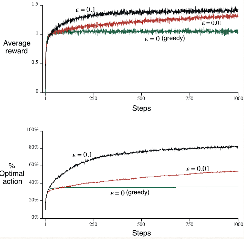 从normal distribution中sample，返回的reward variance为1，1000个time step。greedy收敛快，但是陷入局部最优。greedy可以在1/3的task中找到最优； explore最多，通常更快找到最优解，但是选择的概率没超过91%； 收敛很慢，但最终结果比 好。慢慢减小 是合理的方法。-greedy的效果取决于tasks，若没noise，则greedy最好。若task是nonstationary，true value随时间变化，则我们一直需要explore。nonstationarity是RL中最常见的问题。

2.4 Incremental Implementation

现在考虑如何用constant memory和constant per-time-step computation来计算sample average。考虑single action。 表示第i次得到的这个action的reward， 表示n-1次后这个action的estimated value， incremental formula来计算average，就很剩memory，只需要存 ： (2.3)在本书中很常见，一般的形式是： 是estimate中的error部分，让estimation接近target，如bandit中接近true reward。 step-size parameter， 描述每一步的变化，在bandit中为 。本书中用 或者 表示 。

2.5 Tracking a Nonstationary Problem

之前研究的都是stationary bandit problem，reward probabilities不变。RL中更常见的是nonstationary，给最近的reward更多权重就很合理。其中一个常见的方法是将step-size parameter设为constant： 此时 称为weighted average，reward之前的weight decreases exponentially，也称为exponential recency-weighted average。 表示收到第n个action 后的step-size parameter。 时为sample-average method，大数定理下保证converge到true value。但是并不是所有的 都会converge。stochastic approximation theory给我们converge with probability 1的条件： 第一个条件保证step足够大来克服initial condition。第二个条件保证step足够小来converge（好的完全不懂，我不配）。两个条件在sample-average中都满足，但在costant情况下，第二个条件不满足，所以永远不会converge，一直在根据最新的reward在波动，也是nonstationary情况中我们想要的。满足(2.7)的step-size parameter一般converge很慢且很需要tuning。满足条件的step-size parameter在理论工作中很常见，但很少实用。

2.6 Optimistic Initial Values

之前讨论的都依赖于 ，biased by their initial estimates。对于sample-average，当所有action都被sample至少一次后，bias消失；但对于constant ，bias永远存在，虽然在减小。这种bias也不一定是坏事，甚至有用。虽然需要user来选择，但可以用作prior knowledge。bias可以用于激励exploration。比如在bandit中，设置所有intial value为5，大于所有action的true value，即使用greedy也还可以explore。这种方法称为optimistic initial values，在stationary problem中有用。这些方法都简单，毕竟只是处理一个initial value，有一个用起来就挺好的了。

2.7 Upper-Confidence-Bound Action Selection

对于greedy和epsilon-greedy，更好的方法是选择有potential的action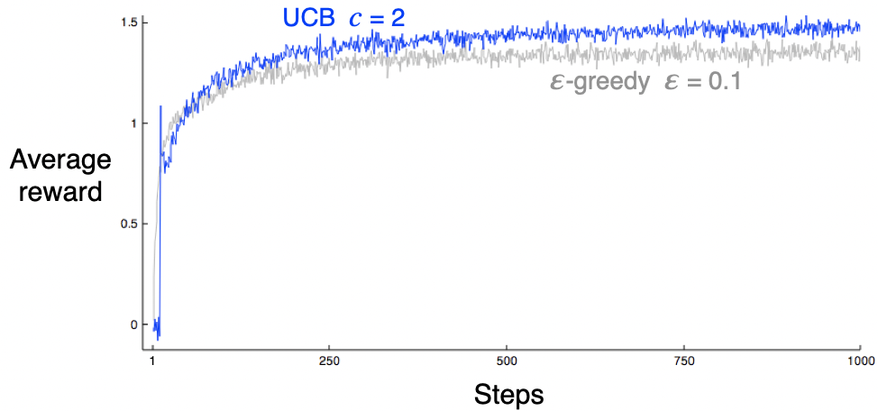： 表示 之前被选择的次数，若为0，即为最大值。 控制exploration。此方法称为upper confidence bound (UCB)，用更号部分表示不确定性， 表示confidence level。UCB的10-arm bandit如图，表现一般都挺好：对于nonstationary problems，需要有比weighted average更复杂的方法。

2.8 Gradient Bandit Algorithms

出了以上估计value和用value选择action的方法，本节学习actions的numerical preference，表示为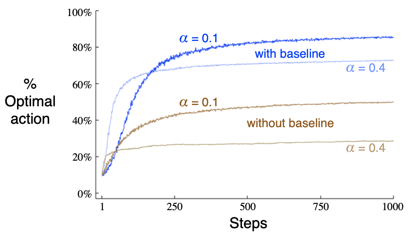 。preference并不是reward的直接表示，而是一个action比其他action相比较的preference，如果每个preference都加1000，选择的概率也不会变，用 来表示： ：the probability of taking action at time 。 ，for all 。两个actions的情况下，用logistic，sigmoid，softmax结果一样一个基于stochastic gradient ascent的更新方法： ：step-size parameter， ：the average of all the rewards up through and including time 。 作为比较reward的basline。10-armed bandit test，mean reward为4P29: bandit stochastic gradient ascent 可以由 gradient ascent 推导。gradient ascent： 。

2.9 Associative Search (Contextual Bandits)

以上都是nonassociative tasks（不同action对于所有state都一样），而常见的RL问题是在不同的state选择最优action。不同action在不同state的true value变化很大，不能使用对应nonstationary problem的方法。associative search task包括trial and error，search for the best actions和association，也称为contextual bandits。此类问题像full RL problem，包括学习一个policy，也想bandit problem，使用immediate reward。

2.10 Summary

本章列了一些平衡exploration and exploitation的简单方法：epsilon-greedy，UCB，gradient bandit algorithm，initializing estimates optimistically。很难评判哪一种方法最好，因为他们都有parameter。下图展示了在10-armed bandit test中parameter和algorithm的关系，这种图称为parameter study。都是在某一个中间值效果最好。总的来说，UCB效果最好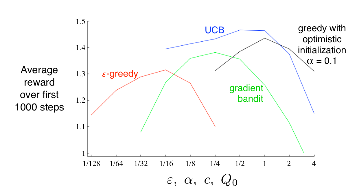虽然本章中的方法都很简单，但其实sota。复杂的方法在实际中难以应用。Gittins indices是平衡exploration and exploitation的一种方法，找到更general bandit problem 的 optimal solution，但要求分布已知，在full RL problem中唔得。Bayesian methods设置initial distribution，然后一步步update，一般来说update的计算很复杂，但对于一些分布（conjugate priors）很简单。这种方法称为posterior sampling 或者 Thompson sampling，一般和不知distribution的方法表现差不多。在Bayesian中，甚至可以计算optimal balance between exploration and exploitation，将distribution也作为问题的information state。给定horizon，我们可以计算所有的可能，但是所有可能的数量也会指数增长。不能精确计算，但可以approximate。